Table of contents

1. Introduction
   1. Improving performance across all abstraction layers
2. Instruction set architectural awareness
   1. Designing an ISA
   2. Further reading
3. Microarchitectural awareness: Pipelining
   1. Pipelining
   2. Exercise 1 - Microarchitecture and Performance
      1. Exercise 1.1
      2. Exercise 1.2
      3. Exercise 1.3
   3. Exercise 2 - Microarchitecture and Performance 2
      1. Exercise 2.1
      2. Exercise 2.2
      3. Exercise 2.3
      4. Exercise 2.4
4. Microarchitectural awareness: Hazards
   1. Data hazards
      1. Exercise 2.5
      2. Forwarding
   2. Exercise 3 - Forwarding
      1. Exercise 3.1
      2. Exercise 3.2
      3. Exercise 3.3
   3. Control hazards
      1. Spectre
   4. Exercise 4 - Code Optimization
      1. Exercise 4.1
      2. Exercise 4.2
   5. Exercise 5 - Branching
5. General architectural awareness
   1. Loop fission
   2. Loop unrolling
   3. Loop tiling

Introduction

The goal of today’s exercise session is to introduce you to some microarchitecture and low-level optimization concepts. Learning about these optimizations will not only make you a better programmer, but will also give you more insight into the wonderful low-level world and enhance your reasoning skills about it. This session covers the material from section 4.1 to 4.8 in the book. If you are unsure about any of the concepts, you can look for it in the book first.

Ripes: To help you solve and reason about the upcoming exercises, it is advised to install the Ripes RISC-V simulator from this GitHub page. There is support for Windows, Mac and Linux. On Ubuntu, make the .AppImage file executable using the command chmod +x <ripes-filename> to run the simulator.

Using Ripes, you can simulate different processors: a single-cycle, and different pipelined RISC-V cores. It also has a great cache simulator, which can help you better understand what was learned in the last session about caches. All programs presented in this session can be executed cycle per cycle using Ripes.

Improving performance across all abstraction layers

Improving runtime performance of software can be done at multiple layers across the computing stack. Below, you see a figure of the abstraction layers we can consider in the context of computing, and some possible performance optimizations that can be applied at each layer. Starting from the top, maybe the most obvious optimizations to you at this point are optimizations of your code, i.e., optimizations of algorithms. While these are an important piece of the optimization puzzle, we will not look at them in the context of CASS.

Going down the stack, two performance improvements happen at the programming language level. The choice of programming language and the optimizations that are done at the assembly level by the compiler may have great impact on the runtime of a function. You have already seen glimpses of this when doing tail recursion in session 3. Smart choices on assembly level may have great impact on the performance of the code, even if on the higher level, the algorithm may stay the same.

In this session, we will focus on three topics that go across different layers in the abstraction:

• Instruction set architectural (ISA) awareness
• Microarchitectural awareness
• Architectural awareness

In instruction set architectural awareness we shortly explain how an ISA can impact the runtime of code. In the main part of this session we will talk about microarchitectural awareness. You have already seen caches in the last session and will now learn about pipelining, out-of-order execution, and what issues arise in this context. Lastly, we will also shortly discuss some general architectural awareness across multiple layers from the choice of programming language down to the microarchitecture, concerning the design of memory accesses and the order of operations.

Instruction set architectural awareness

Before we delve into the details of instruction set architectures, remember the core principle of the CPU clock: The CPU is driven by a clock that switches between two voltages (high and low). The time it takes for the clock to complete one cycle of high and then low voltage is known as the clock period.

When we talk about the runtime of a program, we can look at the general formula below: The time it takes to run a program depends on the number of instructions, the cycles that each instruction takes, and finally the time that each cycle takes. Improving the performance runtime of a program can now be done by decreasing either of these components: Reducing the number of instructions that are needed, reducing the cycles per instruction, or reducing the time per cycle.

Designing an ISA

When creating a new ISA, a design principle decision comes at the very beginning of the process: should programs consist of

1. few specialized instructions or
2. many instructions that are more general?

In short, should the ISA provide (1) a large number of specialized, but complex, instructions that may execute for a longer time or (2) a small set of simple and general instructions that are also faster to execute? This design decision stands behind the difference between CISC vs RISC.

CISC (Complex instruction set computer) designs have been the dominant design for a large time of computing history, mostly because of the popular x86 ISA which is used by Intel and AMD. CISC instructions can be very specialized but also take a longer time to execute. One good example is the x86 instruction REPNE SCASB. This complicated instruction can be used to calculate the size of a string with one line of assembly code. However, the runtime of this instruction obviously depends on the size of the string.

RISC (Reduced instruction set computer) designs like RISC-V or ARM decided that it is better to have a smaller number of instructions that run faster. Programs in RISC will therefore consist of more instructions to achieve the same functionality than a program written in a CISC ISA. For example, to calculate the size of a string in a RISC program, you would loop over the string manually and compare each new character to the null byte. In RISC ISAs, each instruction often takes the same number of cycles to complete, which allows for many simplifications in the CPU and along the data path.

Further reading

CISC vs RISC is an old dilemma that you can also read up a lot on via other sources. Here is a good Stanford website explaining the tradeoffs. Here is a rebuttal statement that it is actually not all that important as people think. In the end, the details of CISC vs RISC are only important to you if you want to design new architectures, but it is important to know that these tradeoffs exist and different architectures have different underlying design philosophies.

The recent ARM chips developed by Apple are RISC CPUs that in some ways outperform their CISC competition from Intel. This means that the battle of CISC vs RISC is definitely not decided yet and will stay relevant over the next years.

Microarchitectural awareness: Pipelining

RISC-V instructions typically take 5 steps to execute:

1. Instruction fetch: fetch the instruction from memory and increment the program counter so that it points to next instruction (pc = pc + 4)
2. Instruction decode: decode the instruction and read the operand registers
3. Execute: execute the operation or calculate the address (for a memory operation)
4. Memory access: when needed, reads operand values from the data memory
5. Write back: write the result into a register

In a single cycle processor implementation, illustrated below, each instruction is executed in one cycle, meaning that these 5 steps happen in a single clock cycle. This also means that the clock cycle must have the same length for all instructions, since the clock frequency cannot dynamically change for each instruction. Therefore, the clock has to be stretched to accommodate the slowest instruction (i.e., it has to be slow enough to allow the slowest instruction to fully execute, from the fetch to the write back step). In other words, even if an instruction could in theory execute faster (e.g., an add could in theory execute faster than a load because it does not need to go through the memory access step), it is limited by the clock speed, which itself is limited by the worst-case instruction.

The performance of such a single cycle processor is therefore constrained by the worst-case instruction. This becomes really problematic when the instruction set contains complex instructions like floating-point operations. In particular for CISC architectures the performance penalty would be completely unacceptable.

Pipelining

Nowadays, almost all processors use an optimization called pipelining. The execution is divided into pipeline steps, called stages, which are operating in parallel. Coming back to our 5-step design: each step corresponds to one pipeline stage and takes one cycle to execute, as illustrated below. The processor can execute the stages in parallel instead of waiting for an instruction to go through all the stages like in a single-cycle design.

0/0

Pipelining does not increase the time to execute a single instruction (called the latency), but increases the number of instructions that can be executed simultaneously and thus the rate at which instructions are executed (called the throughput). In the best case scenario, this five stage pipeline is five times faster than the single-cycle processor:

Exercise 1 - Microarchitecture and Performance

In this exercise, we examine how pipelining affects the clock cycle time of the processor. Solve the following questions both for data paths a and b, assuming that the individual stages of the data paths have the following latencies:

	IF	ID	EX	MEM	WB
a	300ps	400ps	350ps	500ps	100ps
b	200ps	150ps	120ps	190ps	140ps

Exercise 1.1

What is the clock cycle time in a pipelined and single-cycle non-pipelined processor?

Solution

In a pipelined processor, each pipeline stage executes for one clock cycle. This means that the clock cycle needs to be adjusted to accommodate the most time-consuming pipeline stage.

In a single-cycle design, the entire execution with all stages executes in one clock cycle. Naturally, the clock cycle then needs to be as long as the sum of all the stages.

	Pipelined	Single-cycle
a	500ps	1650 ps
b	200ps	800ps

Exercise 1.2

What is the total latency of a lw instruction in a pipelined and single-cycle non-pipelined processor?

Solution

The total latency of an instruction is the time it takes between when the instruction starts to be fetched until its results are written back into memory – in other words, the sum of all stages of execution.

In a pipelined processor, this equals the cycle time multiplied with the number of pipeline stages. In a single-cycle processor, this is simply the cycle time, as all stages execute during one cycle.

	Pipelined	Single-cycle
a	2500ps	1650ps
b	1000ps	800ps

Exercise 1.3

If we can split one stage of the pipelined data path into two new stages, each with half the latency of the original stage, which stage would you split and what is the new clock cycle time of the processor?

Solution

As the cycle time is determined by the most time-consuming stage, this is the one that is worth splitting up. The new cycle time will be determined by the new longest stage.

	Stage to split	New clock cycle time
a	MEM	400ps
b	IF	190ps

Exercise 2 - Microarchitecture and Performance 2

Consider a processor where the individual instruction fetch, decode, execute, memory, and writeback stages in the datapath have the following latencies:

IF	ID	EX	MEM	WB
150ps	50ps	200ps	100ps	100ps

We assume a classic RISC instruction set where all 5 stages are needed for loads (lw), but the writeback WB stage is not necessarily needed for stores (sw) and the memory MEM stage is not necessarily needed for register (R-format) instructions. Instead of a single-cycle organization, we can use a multi-cycle organization where each instruction takes multiple clock cycles, but one instruction finishes before another is fetched. In this organization, an instruction only goes through stages it actually needs (e.g., sw only takes four clock cycles because it does not need the WB stage). Compare clock cycle times and execution times with single-cycle, multi-cycle, and pipelined organization.

Exercise 2.1

Calculate the clock cycle time for a single-cycle, multi-cycle, and pipelined implementation of this datapath.

Solution

The cycle times of the single-cycle and the pipelined processor can be calculated as before, and they will be 600ps and 200ps, respectively.

In the multi-cycle organization, same as for the traditional pipelined design, the clock cycle is limited by the longest stage, so the cycle time of this processor is also minimum 200ps.

In short:

• single-cycle: minimum 600ps
• multi-cycle: minimum 200ps
• pipeline: minimum 200ps

Exercise 2.2

What are the best and worst case total latencies for an instruction in each of the 3 designs (single-cycle, multi-cycle, pipelined)? Express instruction latency both in number of cycles and in total time (ps). Based on these numbers, which design would you prefer? Explain.

Solution

For the single-cycle and the pipelined design, all instructions take the same amount of time regardless of which stages are used during their execution. In the case of the single-cycle processor, this is 600ps (1 cycle), for the pipelined processor, it is 1000ps (5 cycles, each taking 200ps).

In the multi-cycle processor, register instructions don’t use the MEM stage, which means they only have to pass through 4 pipeline stages (4 cycles), adding up to 800ps. For some instructions though, all of the stages are used, so in the worst case the execution takes 1000ps.

The single-cycle and the multi-cycle designs outperform the pipelined design in terms of instruction latency, but due to the parallel nature of the pipelined design, that one still performs much better in terms of instruction throughput. This is demonstrated by the following exercise.

In short:

• single-cycle: always the same: 1 cycle (600ps)
• multi-cycle: best case (R-format) = 4 cycles (4200=800ps), worst case = 5 cycles (5200=1000ps)
• pipeline: always the same: 5 cycles (5*200=1000ps)

Exercise 2.3

Consider the following RISC-V program:

addi t0, zero, 10
sw zero, 4(t1)
lw t2, 10(t3)

For each of the 3 CPU designs (single-cycle, multi-cycle, pipelined), fill out the grid below where the horizontal axis represents time (every cell is 100 ps), and the vertical axis lists the instruction stream. First draw the clock signal indicating at which time intervals a new CPU cycle starts, and then visualize how the processor executes the instruction stream over time. Clearly indicate the start and end of each of the 5 datapath stages (IF, ID, EX, MEM, WB) for all instructions. Note: you can assume the CPU starts from a clean state (e.g., after a system reset).

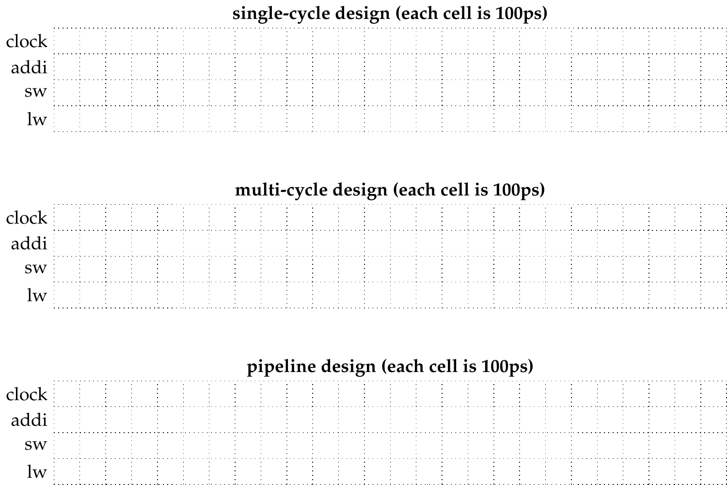
Solution

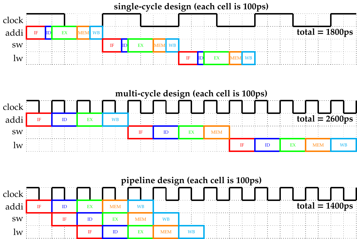
From these figures, we can see how much more efficient the pipelined design is, even for shorter programs.

Exercise 2.4

What is the total time and cycles needed to execute the above RISC-V program from question 2.3 for each of the three CPU designs? What if we add 50 no-operation (nop) instructions (add zero, zero, zero)? Provide a formula to explain your answer.

Solution

For the single-cycle design, the original program takes 3 cycles to execute, which is 3 * 600ps = 1800ps. As every instruction takes 600ps to execute, adding the nop instructions would result in an additional 50 * 600ps = 30,000ps.

In the multi-cycle system, the original program took 13 cycles, as the first two instructions need 4 cycles each, the third one needs all 5. This gives a total execution time of 13 * 200ps = 2600ps. Nop instructions do not access the memory, so they execute for 4 cycles. This means that adding the 50 extra instructions would increase the execution time by 50 * 4 = 200 cycles, which equals 200 * 200ps = 40,000ps.

For the pipelined processor, the first instruction takes 5 cycles to execute. During this time, the pipeline already starts executing the next instructions, and after the 5th cycle, one instruction finishes in every cycle. As a result, the example program finishes in 7 cycles, 7 * 200ps = 1400ps. If we add 50 nop instructions, those extend the execution time with 50 cycles, as in each cycle one nop instruction will complete, resulting in an extra time of 50 * 200ps = 10,000ps.

In short:

• single-cycle: 3 cycles (1800ps); 50 extra cycles (+30,000 ps)
• multi-cycle: 13 cycles (2600ps); 50*4 extra cycles (+40,000 ps)
• pipeline: 7 cycles (1400ps); 50*1 extra cycles (+10,000 ps)

Microarchitectural awareness: Hazards

While pipelining is great for parallelizing operations and speeding up instructions by performing multiple operations in a single clock cycle, it may also lead to problems. Specifically, when an operation that we want to perform relies on an operation that has not happened yet or that has only just completed, we speak of a hazard. There are three types of hazards:

• Structural hazards occur when instructions in different stages of the pipeline need access to the same resource in the same cycle, for example, if the instruction fetch stage uses the same memory bus as the memory stage. In pipelined RISC-V processors this hazard usually doesn’t occur (e.g., instructions can be fetched in the same cycle as when memory loads are executing).
• Data hazards occur when an operation relies on data that is yet to be provided by an earlier operation. The easiest example is using the result of an addition that is yet to be written to a register.
• Control hazards arise when decisions need to be taken based on branches that are not yet resolved. The easiest example is a conditional branch where the CPU must already decide what instruction it loads next before knowing what the result of the conditional branch is.

In this session we will now look at data and control hazards.

Data hazards

The figure below shows a simple data hazard. The addi instruction will only write the new value of the register back into t0 in the WB stage. However, lw will already need the correct value in the EX stage which occurs one cycle before, leading to a data hazard.

There are three basic data dependencies that indicate a data hazard:

• Read after write (RAW): Data, which is read after it was previously written. Here, the old value of the data may be read before the new one is written.
• Write after read (WAR): Data is written after it was read earlier. In some pipelines and optimizations, the “later” write may already affect the earlier read.
• Write after write (WAW): Two writes may conflict with each other.

Exercise 2.5

Recall the RISC-V program from above.

addi t0, zero, 10
sw zero, 4(t1)
lw t2, 10(t3)

Describe the performance implications for each of the three CPU designs from exercise 2, if in the RISC-V program the first instruction is changed to addi t1, zero, 10 (think about hazards).

Solution

As there is no parallelism in single-cycle and multi-cycle processors, there are also no hazards. Instructions only start executing once the previous once have completely finished and their modifications have been carried out in memory or the register file.

In the pipelined design, changing the first instruction like this would create a read after write (RAW) dependency between the first and the second instructions, as the second one uses the t1 register the first instruction writes to. The second instruction needs the correct value of t1 in its EX stage, but by then the first instruction is only in its MEM stage, the register file has not been written yet. To avoid this hazard, the processor either has to stall the second instruction until the correct value is available in t1 or set up data forwarding between the pipeline registers.

Forwarding

Data hazards can be a big problem if not accounted for. The simplest way to deal with them is to add enough nop instructions before each data hazard to ensure that the information is available before the hazard may occur. Another approach is to cleverly reorder instructions so that hazards can be avoided. This must obviously be done in a way that does not change the result of the computation and can only work in a limited subset of occasions.

To tackle data hazards more structurally, a CPU pipeline can forward information once it becomes available to the next or an earlier stage. This prevents specific data hazards from occurring. Below, you see a simple forwarding mechanism from the EX stage to the EX stage that forwards the new value of a register to immediately be available for the lw instruction in the next cycle.

While forwarding like this has many benefits, it also has limitations. Below, you see one example where forwarding cannot help because the information of lw only becomes available in the MEM stage, which happens at the same time when the next instruction, addi, requires it in the EX stage.

The only way to deal with this is to stall the current execution (also called inserting a bubble), and let the processor wait until the information becomes available. This is equivalent to inserting a nop (no operation) instruction between the instructions causing the hazard. Simply said, if the information becomes available in the same cycle that it is needed, there is nothing we can do with forwarding and we instead have to stall. Below you see a solution to this problem with stalling and a forwarding from the MEM stage to the EX stage.

Exercise 3 - Forwarding

The code below describes a simple function in RISC-V assembly.

or t1, t2, t3
or t2, t1, t4
or t1, t1, t2

Exercise 3.1

Indicate the dependencies in the code and their type: read after write (RAW), write after read (WAR), write after write (WAW).

Solution

• Both (2) and (3) read t1 after (1) writes it (RAW)
• (3) reads t2 after (2) writes it (RAW)
• (2) writes t2 after (1) reads it (WAR)
• (3) writes t1 after (2) reads it (WAR)
• (3) writes t1 after (1) writes it (WAW)

Exercise 3.2

Assume there is no forwarding in the pipelined processor. Indicate hazards and add nop instructions in the program to eliminate them.

Solution

WAR and WAW dependencies do not cause hazards in the pipeline; it does not matter what the value of the register is when it is being written.

RAW dependencies cause hazards for two instructions that follow the instruction that writes the value.

1	2	3	4	5	6	7	8
IF	ID	EX	ME	WB				(1)
	IF	ID	EX	ME	WB			(2)
		IF	ID	EX	ME	WB		(3)
			IF	ID	EX	ME	WB	(4)

If instruction (1) writes a register value, that write will happen in clock cycle 5, in the WB stage. The earliest that value can be read is in the same clock cycle. (Writes to the register file happen in the first half of the cycle, reads in the second, this is why it’s possible to read the correct value in the same cycle it gets written.)

As register values are read in the ID stage, that means that instructions (2)-(3) would still load the stale register value, they either need to be stalled or the correct value needs to be forwarded to their EX stage.

In this case, we manually stall instructions by inserting nops to mitigate the two RAW hazards:

or t1, t2, t3
nop
nop
or t2, t1, t4
nop
nop
or t1, t1, t2

Exercise 3.3

Assume there is full forwarding in the pipelined processor. Indicate the remaining hazards and add nop instructions to eliminate them. Compared the speedup achieved by adding full forwarding to a pipeline with no forwarding.

Assume the following cycle times for two processors with different forwarding strategies:

• Without forwarding: 250ps
• With full forwarding: 300ps

Solution

With full forwarding, register values that are calculated in the EX stage can be forwarded to the following instruction’s EX stage, which eliminates the hazards in this code. This means that we don’t need to add any nop instructions.

The execution time for this program is 7 cycles, 5 to execute the first instruction and 2 to finish the other two. With the increased cycle time, this amounts to 7 * 300ps = 2100ps.

Without forwarding, we are forced to add the 4 nop instructions, which adds 4 additional cycles to the execution time. Even with the shorter cycle times, this is (7+4) * 250ps = 2750ps, which is 1.3 times longer than with full forwarding.

Control hazards

Control hazards happen when the proper instruction cannot execute in a pipeline stage because the instruction that was fetched is not the correct instruction. The easiest example is a conditional branch where the CPU must start fetching next instructions before actually knowing the outcome of the conditional branch.

A first solution would be to stall the pipeline until the outcome of the conditional branch is known, and we know which instructions to fetch. Unfortunately, this solution incurs a penalty on every branch, which might become too high when the outcome of the branch cannot be decided quickly.

An optimization, featured in most processors, is to try to predict the outcome of a branch. For instance, the processor can predict that branches are never taken and start fetching and executing corresponding instructions as shown in the following example:

If the prediction is correct, we have a performance gain and the pipeline proceeds at full speed. If the prediction is incorrect, we have to discard the wrongly executed instructions in the pipeline (which is called a pipeline flush) and resume execution along the correct branch as shown in the following example. Of course, we must make sure that these incorrect sequences of instructions (called transient executions) can be reverted (for instance, they must not write to memory). In this case, the penalty is roughly equivalent to stalling.

Such prediction mechanisms are called speculative execution and are implemented in almost all processors. Modern processors have more sophisticated prediction mechanisms that can be updated dynamically. For instance, such a branch predictor could remember whether a particular branch was recently taken or not, and base its prediction on this. Speculative execution can also be applied to predict the outcome of indirect branches or ret instructions.

You might be wondering what the difference between speculative execution and transient execution is. Speculative execution is any sequence of instructions that is executed by the processor after a prediction (and before the prediction is resolved). In particular, the processor does not know if speculatively executed instructions will be committed or flushed. Transient executions specifically refer to incorrectly executed instructions. In particular, transient executions can happen because of speculative execution, but speculative execution is not the only source of transient execution.

Spectre

In 2018, a major vulnerability called Spectre became public, which has been discovered jointly by academic and industry security researchers. The vulnerability had a tremendous impact not only on academic research but also on industry: mitigations were proposed for microprocessors, operating systems, and other software. With our knowledge about architectures (speculative execution in particular) we can now understand what happened!

The main idea behind Spectre attacks is to exploit prediction mechanisms in order to leak secrets to the microarchitectural state during transient execution. Transient executions are reverted at the architectural level (they do not impact the final value of registers or memory) but their effect on the microarchitectural state (for instance the cache) is not reverted. This means that if a secret is accessed during transient execution, computations on that secret can leave traces in the microarchitecture. For instance, if a secret is used as an index to load data from memory (load[secret]), the state of the cache will be affected by the value of secret, and an attacker can use cache attacks to retrieve the value of that secret.

Consider for instance the following code where an attacker wants to learn the value of secret but cannot directly access it: they can only call the function spectre_gadget with an arbitrary value i. Notice that the program is protected against cache attacks because the secret cannot be used as a memory index during “normal” (non-transient) execution.

int tab[4] = { 0, 1, 2, 3 };
char tab2[1024];
int secret; // The secret we want to protect

void spectre_gadget(int i) {  // The attacker calls the function with i=260
   if (i < 4) {               // The condition mispeculated
    int index = tab[i];       // index = secret
    char tmp = tab2[index * 256]; // secret is used as a load index during transient execution
    // [...]
   }
}

1. The attacker can (optionally) train the branch predictor so that it predicts the condition (i < 4) to be true;
2. The attacker prepares the cache (e.g., by flushing the content of tab2);
3. The attacker calls the victim with a value i such that tab[i] returns the secret. Remember how pointer arithmetic works: tab[i] = tab + i * 4. Additionally, notice that secret is located at address tab + 1024 + 4*4. Hence, we need to find i such that tab + i * 4 = tab + 1024 + 4*4, which is achieved with i = 260. In other words, index = tab[260] will load secret in index if the branch is mispredicted to be true!
4. The processor predicts the branch to be true, accesses the secret and uses it as an index to access tab2, which brings tab2[secret] into the cache. The processor eventually realizes that the prediction is incorrect and flushes the pipeline, but the state of the cache is not reverted.
5. Finally, the attacker can use cache attacks (like in the previous session) to infer which cache lines have been accessed by the victim and recover the value of secret!

The Spectre attack illustrated above abuses the conditional branch predictor, but there exist other variants of Spectre that exploit different prediction mechanisms.

Exercise 4 - Code Optimization

The code below describes a simple function in RISC-V assembly (A = B + E; C = B + F).

lw t1, 0(t0)
lw t2, 4(t0)
add t3, t1, t2
sw t3, 12(t0)
lw t4, 8(t0)
add t5, t1, t4
sw t5, 16(t0)

Exercise 4.1

Assume the program above will be executed on a 5-stage pipelined processor with forwarding and hazard detection. How many clock cycles will it take to correctly run this RISC-V code?

Solution

In this code, both add instructions will have to be stalled for one cycle. Both of them have a RAW dependency on a register value that is loaded from memory in the previous instruction. This value is only available in the MEM stage of the lw instruction, which runs in parallel with the EX stage of the add instruction. For this reason, the add instructions need to be stalled by one cycle, so that the correct register value can be forwarded to their EX stages.

Inst	1	2	3	4	5	6	7
lw	IF	ID	EX	ME	WB
add		IF	ID	XXXX	EX	ME	WB

In total, this means that we have 5 cycles for the first instruction, 6 (1 each) for completing the additional instructions, and 2 due to the two stalls. 5 + 6 + 2 = 13

Exercise 4.2

Reorganize the code to optimize the performance. (Hint: try to remove the stalls)

Solution

If we avoid using a register value in an instruction that is loaded from memory in the previous instruction (without changing the result of the program), we can eliminate the stalls.

lw t1, 0(t0)
lw t2, 4(t0)
lw t4, 8(t0)
add t3, t1, t2
sw t3, 12(t0)
add t5, t1, t4
sw t5, 16(t0)

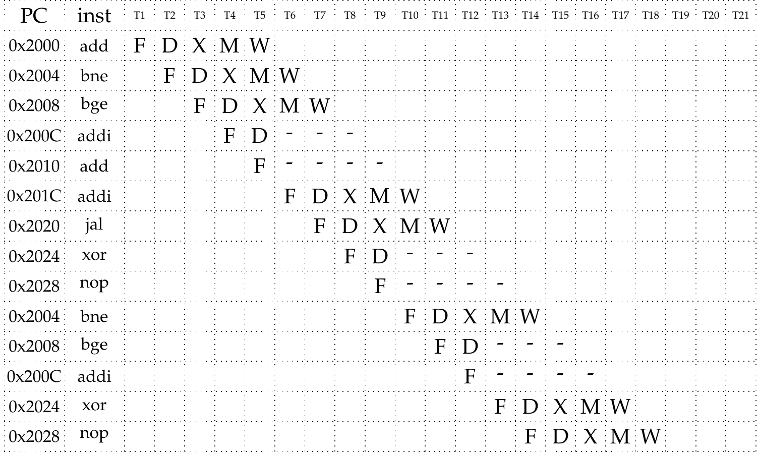
Exercise 5 - Branching

The code below describes a simple function in RISC-V assembly.

      add t0, zero, zero
bar:
      bne t0, zero, exit
      bge t0, zero, foo
      addi t0, t0, -100
      add t1, t1, t1
      add t2, t0, t0
      sub t0, t0, t3
foo:
      addi t0, t0, 1
      jal bar
exit:
      xor s0, s1, s2
      nop

Fill out the following instruction/time diagram for this program until the instruction on line 13 (xor) fully executes and commits. Assume that the processor features data forwarding but does not feature branch prediction: it simply continues executing instructions that follow a branch until the target of the branch is known. Execution starts from the first add instruction with PC=0x2000.

Solution

In this exercise, we need to pay attention to branches and jumps. The processor does no prediction, so it continues executing instructions that follow the branch instruction. The program counter is updated in the EX stage of the branch instructions, so the fetching of the correct next instruction can only start after this stage finished executing. This means that after each branch that is taken, the processor starts executing two incorrect instructions. These executions need to be stopped, the pipeline is flushed after the program counter updates.

General architectural awareness

As final content for the exercise sessions, we will explain some general methods one can apply to make use of a CPU architecture. These may be the most applicable performance optimizations you can think of later in your programming career. Very often, compilers and interpreters may already perform similar optimizations for you, so you may not see any immediate benefit when applying these optimizations. However, sometimes there can be a huge performance increase if one helps the compiler out.

In general, the modern rule of thumb should be to not attempt optimizations by oneself but first let the compiler and its tools give it a try. Usually, the generic approaches of optimizing code are already very sophisticated. However, when specific code optimizations are needed, it is useful to have the understanding of the lower-level principles and the architecture that you now have, to methodologically attempt to make specific performance improvements to select pieces of code.

Loop fission

Due to the principle of locality, we know that accesses that are close to each other in memory may be faster than varying accesses at the same time. Sometimes, it may be faster to break a loop into multiple loops over the same index range and allow each new loop to focus on only parts of the original loop’s body. This can improve locality of reference for both data (the different arrays don’t evict each other from the cache) and code (the entire code of the loop can fit in the instruction cache) since the microarchitecture can kick in optimizations at the hardware level. Below you see a simple example of this where instead of accessing both arrays in the same loop, we split up the loop and run it twice.

example code	with loop fission
int i, a[100], b[100]; for (i = 0; i < 100; i++) { a[i] = 1; b[i] = 2; }	int i, a[100], b[100]; for (i = 0; i < 100; i++) { a[i] = 1; } for (i = 0; i < 100; i++) { b[i] = 2; }

Loop unrolling

In a similar vein, very short loops may suffer from a lot of overhead due to the conditional branch that performs the loop. Sometimes decreasing the actual amount of instructions may be beneficial since it results in fewer jumps or conditional branches and can be beneficial for the pipeline. As you may guess, this optimization method also has the great potential of actually performing worse due to the microarchitecture!

example code	with loop unrolling
for (int i=0; i<N; i++) { sum += data[i]; }	/* assume N is a multiple of 4 */ for (int i=0; i<N; i+=4) { sum1 += data[i+0]; sum2 += data[i+1]; sum3 += data[i+2]; sum4 += data[i+3]; } sum = sum1 + sum2 + sum3 + sum4;

Loop tiling

Lastly, the access pattern of a loop can be optimized by processing the loop in chunks instead of over the whole range repeatedly. This Wikipedia article explains the concept well. Essentially loop tiling aims to decrease the number of cache misses during the processing of a loop which can decrease runtime considerably.